Introduction to OpenJij Core Interface

This tutorial explains how to use OpenJij’s core interface (core python interface).

The core interface is a low-layer API than the previous tutorials. The readers are assumed to have gone through the previous OpenJij tutorials and to be familiar with terms such as Ising models and Monte Carlo methods.

The purpose of the core interface are:

• To use OpenJij for more specialized applications such as sampling and research applications as well as optimization problems.

• To set up annealing schedules

• To directly modify the algorithms

About the OpenJij Core Interface

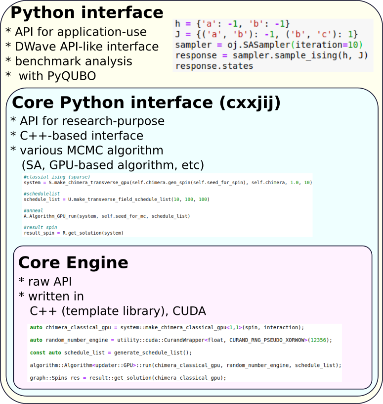
In the previous tutorials, we introduced how to solve various problems using OpenJij and how to benchmark it. OpenJij is implemented in C++ based on the Markov Chain Monte Carlo (MCMC) method, which is a numerical computation method in statistical physics. The Python modules mentioned so far call openjij.cxxjij, a python library that directly wraps this C++ interface. The diagram shows the following inclusions.

The OpenJij core interface allows you to use all the functionality on OpenJij. Thus, it can be used not only for optimization problems but also for research purposes as a numerical tool for statistical physics. The C++ interface allows for faster operations.

This tutorial introduces openjij.cxxjij, a more user-friendly Python interface. pip is used for installation.

Overview of OpenJij Core Interface

First, to see how to use the OpenJij core interface, let us solve the classical spin ($\sigma = \pm 1$) Ising problem with variable size $N=5$ using simulated annealing. The Hamiltonian is as follows:

$$\begin{align*} H &= \sum_{i<j}J_{ij}\sigma_i \sigma_j + \sum_{i=1}^{N}h_i \sigma_i \\ \sigma_i &= \pm 1 (i=1 \cdots N) \end{align*}$$

We set the longitudinal magnetic field and the interaction to be:

$$\begin{align*} h_i = -1 \ \mathrm{for\ } \forall i,\ J_{ij} = -1　\ \mathrm{for\ } \forall i,\ j \end{align*}$$

$\{\sigma_i\} = \{1,1,1,1,1,1\}$ is the optimal solution since each spin has lower energy if it takes the value of 1. Let us solve this problem. The process using Python code is as follows:

The core interface is a specialized solver for Ising problems. To convert to QUBO, please refer to the previous tutorials and convert from QUBO to the Ising problem before calling the core interface.

# import cxxjij instead of openjij
import openjij.cxxjij as cj

# Create the interaction matrix using the Graph module
import openjij.cxxjij.graph as G

# Define a densely connected graph (Dense) with problem size N = 5.
N = 5
J = G.Dense(N)
# Set interactions
for i in range(N):
    for j in range(N):
        #Enter -1 for j[i,i] else
        J[i,j] = 0 if i == j else -1.0

# Set a vertical magnetic field
for i in range(N):
    # J[i,i] = -1 will give the same result
    J[i] = -1

# Create a system to perform the calculation
import openjij.cxxjij.system as S

# We use the usual classical Monte Carlo system
system = S.make_classical_ising(J.gen_spin(), J)
# Set an annealing schedule using the Utility module
import openjij.cxxjij.utility as U
schedule = U.make_classical_schedule_list(0.1, 100, 10, 10)

# Run the annealing using the Algorithm module
# Use a simple SingleSpinFlip to update the Monte Carlo step
import openjij.cxxjij.algorithm as A
A.Algorithm_SingleSpinFlip_run(system, schedule)

# Get the result using get_solution in the Result module
import openjij.cxxjij.result as R
print("The solution is {}.".format(R.get_solution(system)))

The solution is [1, 1, 1, 1, 1].

The answer that comes out is $[1,1,1,1,1,1]$. There are many items to be configured for the low-layer API, but this allows for a more detailed configuration.

Module List

As shown in the code example, the OpenJij core interface mainly consists of modules such as graph, system, updater, algorithm and result. By combining these modules, it is possible to compute the Ising model with various types and algorithms. The modules can be easily extended to implement new algorithms. A detailed explanation will be given in the following notebooks.

Graph

This module is used to store the coefficients $J_{ij}$ of the Ising Hamiltonian. Dense deals with tight coupling (suitable for models where all $J_ij$ have non-zero values), and Sparse deals with sparse coupling (suitable for models where many of the $J_ij$ values are zero).

System

The system defines a data structure to hold the current system state for Monte Carlo and other calculations such as:

• Classical Ising model (spins)

• Transverse field Ising model (spins including Trotter decomposition)

• GPU-implemented classical and quantum Ising models

There are (and/or will be) a variety of Monte Carlo and other computational methods. Therefore, OpenJij is designed to facilitate the addition of various algorithms by separating the data structures and algorithms for each method and the interface for retrieving the results.

Updater

This defines how the system is to be updated such as:

• SingleSpinFlip Update

• SwendsenWang Update

The Updater that can be used is determined by the type of System. The specific types of updaters that can be used on each system type will be discussed in the following tutorials.

In the core python interface, it is integrated into algorithm.

Algorithm

It is responsible for running the algorithm, including what schedule to run the annealing algorithm using updater. It can be run using the corresponding updater at Algorithm_[Updater type]_run.

Result

This is used to get information from system, such as spin configuration.

Coding Flow

The coding flow is shown below. This flow does not change even when the scale of the problem grows.

• Define $J_{ij}, h_{i}$ in the graph module

• Create system based on the graph module

• Select updater corresponding to system and run the algorithm with Algorithm_[Updater type]_run

• Get the spin configuration of the system with result.get_solution(system) or directly from system