Clique Cover Problem

Here we show how to solve the clique cover problem using OpenJij, JijModeling, and JijModeling Transpiler. This problem is also mentioned in 6.2. Clique Cover in Lucas, 2014, “Ising formulations of many NP problems”.

Overview of the Clique Cover Problem

The clique covering problem is to determine whether, given a graph and an integer $n$, the graph can be partitioned into $n$ cliques (complete graphs).

Complete Graph

A complete graph is a graph whose two vertices are all adjacent to each other (not including loops or multiple edges). We show two examples below.

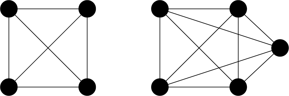
As mentioned, a vertex in a complete graph is adjacent to all other vertices. A complete undirected graph $G = (V, E)$ has ${}_V C_2 = \frac{1}{2} V(V-1)$ edges, which shows that the number of edges is equal to the number of combinations choosing two vertices from $V$. Based on minimizing the difference in the number of edges from a complete graph, we describe a mathematical model for the clique cover problem.

Binary Variable

We introduce a binary variable $x_{v, n}$ such that $x_{v, n}$ is 1 if the vertex $v$ belongs to the $n$th clique and 0 otherwise.

Constraint

Each vertex can belong to only one clique, meaning that the graph is divided into $N$ cliques:

(1)$$\sum_{n=0}^{N-1} x_{v, n} = 1 \quad (\forall v \in V)$$

Objective Function

Let us consider the $n$th subgraph $G (V_n, E_n)$. The number of vertices is $V_n = \sum_v x_{v,n}$. If this subgraph is complete, the number of edges of this subgraph is $\frac{1}{2} V_n (V_n -1)$ from the previous discussion. The number of edges can actually be written as $\sum_{(uv) \in E_n} x_{u, n} x_{v, n}$. The subgraph $G$ is neatly divided into cliques when the difference between these two approaches is zero. Therefore, we set the objective function as follows:

(2)$$\mathbf{obj} = \sum_{n=0}^{N-1} \left\{ \frac{1}{2} \left( \sum_{v=0}^{V-1} x_{v, n} \right) \left( \sum_{v=0}^{V-1} x_{v, n} -1\right) - \sum_{(uv) \in E} x_{u, n} x_{v, n} \right\}$$

Modeling by JijModeling

Next, we show an implementation using JijModeling. We first define variables for the mathematical model described above.

Variables

Let us define the variables used in expressions (1) and (2) as follows:

import jijmodeling as jm

# define variables
V = jm.Placeholder('V')
E = jm.Placeholder('E', dim=2)
N = jm.Placeholder('N')
x = jm.Binary('x', shape=(V, N))
n = jm.Element('n', (0, N))
v = jm.Element('v', (0, V))
e = jm.Element('e', E)

---------------------------------------------------------------------------
ModuleNotFoundError                       Traceback (most recent call last)
Cell In[1], line 1
----> 1 import jijmodeling as jm
      3 # define variables
      4 V = jm.Placeholder('V')

ModuleNotFoundError: No module named 'jijmodeling'

V=jm.Placeholder('V') defines the number of vertices in the graph and E=jm.Placeholder('E', dim=2) defines the graph’s edge set. N=jm.Placeholder('N') determines how many cliques the graph is divided into, and V, N is used to define the binary variable $x_{v, n}$ as x=jm.Binary('x', shape=(V, N)). n, v is the variable used to index the binary variable, and e is the variable for the edge. e[0], e[1] are the vertices located at both ends of edge e, which makes $(uv) = (e[0] e[1])$.

Constraints

Let us implement the constraint in expression (1).

# set problem
problem = jm.Problem('Clique Cover')
# set one-hot constraint: each vertex has only one color
problem += jm.Constraint('color', x[v, :]==1, forall=v)

x[v, :] implements Sum(n, x[v, n]) in a concise way.

Objective Function

Let us implement the objective function of expression (2).

# set objective function: minimize the difference in the number of edges from complete graph
clique = x[:, n] * (x[:, n]-1) / 2
num_e = jm.Sum(e, x[e[0], n]*x[e[1], n])
problem += jm.Sum(n, clique-num_e)
problem

$$\begin{alignat*}{4}\text{Problem} & \text{: Clique Cover} \\\min & \quad \sum_{ n = 0 }^{ N - 1 } \left( \frac{ \sum_{ \bar{i}_{0} = 0 }^{ V - 1 } x_{\bar{i}_{0},n} \cdot \left( \sum_{ \bar{i}_{0} = 0 }^{ V - 1 } x_{\bar{i}_{0},n} - 1 \right) }{ 2 } - \sum_{ e \in E } x_{e_{0},n} \cdot x_{e_{1},n} \right) \\\text{s.t.} & \\& \text{color} :\\ &\quad \quad \sum_{ \bar{i}_{1} = 0 }^{ N - 1 } x_{v,\bar{i}_{1}} = 1,\ \forall v \in \left\{ 0 ,\ldots , V - 1 \right\} \\[8pt]& x_{i_{0},i_{1}} \in \{0, 1\}\end{alignat*}$$

With clique, we calculate the number of edges if the vertex had created a clique. The next num_e is the calculated number of edges that the vertex has. Finally, the sum of the differences is added as the objective function.

Instance

Here we prepare a graph using NetworkX.

import networkx as nx

# set the number of colors
inst_N = 3
# set empty graph
inst_G = nx.Graph()
# add edges
inst_E = [[0, 1], [1, 2], [0, 2], 
            [3, 4], [4, 5], [5, 6], [3, 6], [3, 5], [4, 6], 
            [7, 8], [8, 9], [7, 9], 
            [1, 3], [2, 6], [5, 7], [5, 9]]
inst_G.add_edges_from(inst_E)
# get the number of nodes
inst_V = list(inst_G.nodes)
num_V = len(inst_V)
instance_data = {'N': inst_N, 'V': num_V, 'E': inst_E}

The graph set up by this instance is as follows.

import matplotlib.pyplot as plt

nx.draw_networkx(inst_G, with_labels=True)
plt.show()

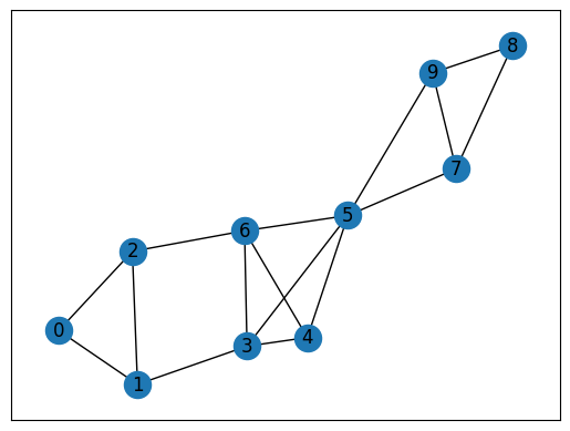
This graph consists of three cliques (0, 1, 2), (3, 4, 5, 6), and(7, 8, 9).

Undetermined Multiplier

This problem has one constraint, and we need to set the weight of that constraint. We will set it to match the name we gave in the Constraint part earlier using a dictionary type.

# set multipliers
lam1 = 1.1
multipliers = {'color': lam1}

Conversion to PyQUBO by JijModeling Transpiler

JijModeling has executed all the implementations so far. By converting this to PyQUBO, it is possible to perform combinatorial optimization calculations using OpenJij and other solvers.

from jijmodeling.transpiler.pyqubo import to_pyqubo

# convert to pyqubo
pyq_model, pyq_chache = to_pyqubo(problem, instance_data, {})
qubo, bias = pyq_model.compile().to_qubo(feed_dict=multipliers)

The PyQUBO model is created by to_pyqubo with the problem created by JijModeling and the instance_data we set to a value as arguments. Next, we compile it into a QUBO model that can be computed by OpenJij or other solver.

Optimization by OpenJij

This time, we will use OpenJij’s simulated annealing to solve the optimization problem. We set the SASampler and input the QUBO into that sampler to get the result of the calculation.

import openjij as oj

# set sampler
sampler = oj.SASampler()
# solve problem
response = sampler.sample_qubo(qubo, num_reads=100)

Decoding and Displaying the Solution

Decode the returned results to facilitate analysis.

# decode solution
result = pyq_chache.decode(response)

From the result thus obtained, let us visualize the graph. By using result.feasible(), only feasible solutions can be extracted. From here, the process of coloring the vertices for each clique is performed.

# extract feasible solution
feasible = result.feasible()
if feasible.evaluation.objective == []:
    print('No feasible solution found ...')
else:
    print("Objective: "+str(feasible.evaluation.objective[0]))
    # get indices of x = 1
    indices, _, _ = feasible.record.solution['x'][0]
    # get vertex number and color
    vertices, colors = indices
    # sort lists by vertex number
    zip_lists = zip(vertices, colors)
    zip_sort = sorted(zip_lists)
    sorted_vertices, sorted_colors = zip(*zip_sort)
    # initialize vertex color list
    node_colors = [-1] * len(vertices)
    # set color list for visualization
    colorlist = ['gold', 'violet', 'limegreen']    
    # set vertex color list
    for i, j in zip(sorted_vertices, sorted_colors):
        node_colors[i] = colorlist[j]
    # make figure
    fig = plt.figure()
    nx.draw_networkx(inst_G, node_color=node_colors, with_labels=True)
    plt.show()

Objective: 0.0

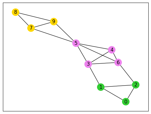
It is correctly divided into cliques. We recommend you try more complex graphs.