6-Machine Learning (QBoost) with Quantum Annealing

In this section, we describe an application of machine learning (ML) with quantum annealing (QA) optimization.

In the first, we show application for clustering task using JijModeling and OpenJij.
In the second, we execute an ensemble study called QBoost with PyQUBO and D-Wave sampler.

Clustering

Clustering is the task of dividing given set of data into $n$ clusters ($n$ is our input). For the sake of simplicity, let us consider the number of cluster $n$ is 2 in this time.

Clustering Hamiltonian

We demonstrate clustering by minimizing the following Hamiltonians.

$$H = - \sum_{i, j} \frac{1}{2}d_{i,j} (1 - \sigma _i \sigma_j)$$

Where $i, j$ is sample No., $d_{i, j}$ is a distance between $i$ and $j$, $\sigma_i=\{-1,1\}$ is spin variable that indicates whether $i$ belong to one of the two clusters.

Each term of this Hamiltonian sum behaves as follows.

• 0 for $\sigma_i = \sigma_j$

• $d_{i,j}$ for $\sigma_i \neq \sigma_j$

Note that minus of R.H.S., Hamiltonian means the problem is “Choosing pairs of $\{\sigma _1, \sigma _2 \ldots \}$ that maximizes the distance between the samples of different classes”.

Importing the required libraries

We import several libraries for clustering.

# import libraries
import numpy as np
from matplotlib import pyplot as plt
import pandas as pd
from scipy.spatial import distance_matrix

import openjij as oj
import jijmodeling as jm
from jijmodeling.transpiler.pyqubo.to_pyqubo import to_pyqubo

---------------------------------------------------------------------------
ModuleNotFoundError                       Traceback (most recent call last)
Cell In[1], line 3
      1 # import libraries
      2 import numpy as np
----> 3 from matplotlib import pyplot as plt
      4 import pandas as pd
      5 from scipy.spatial import distance_matrix

ModuleNotFoundError: No module named 'matplotlib'

Clustering with JijModeling and OpenJij

At first, we formulate the mathematical model in JijModeling. We cannot use spin variable in JijModeling, so we change spin variable $\sigma_i$ to binary variable $x_i$ by using the relationship $\sigma_i = 2x_i - 1$.

problem = jm.Problem("clustering")
d = jm.Placeholder("d", dim=2)
N = d.shape[0]
x = jm.Binary("x", shape=(N))
i = jm.Element("i", (0, N))
j = jm.Element("j", (0, N))
problem += (
    -1 / 2 * jm.Sum([i, j], d[i, j] * (1 - (2 * x[i] - 1) * (2 * x[j] - 1)))
)
problem

$$\begin{alignat*}{4}\text{Problem} & \text{: clustering} \\\min & \quad \left( -0.5 \right) \cdot \sum_{ i = 0 }^{ d_{\mathrm{shape}(0)} - 1 } \sum_{ j = 0 }^{ d_{\mathrm{shape}(0)} - 1 } d_{i,j} \cdot \left( 1 - \left( 2 \cdot x_{i} - 1 \right) \cdot \left( 2 \cdot x_{j} - 1 \right) \right) \\& x_{i_{0}} \in \{0, 1\}\end{alignat*}$$

Make artificial data

Next, we create instance data for the clustering problem.

In this case, let us generate linearly separable data in a two-dimensional plane artificially. Our clustering algorithm is unsupervised learning algorithm, so we do not need to prepare answer data.

data = []
label = []
N = 100
for i in range(N):
    # generate 0 to 1 random number
    p = np.random.uniform(0, 1)
    # set class 1 when certain condition are met, and -1 when it are not met
    cls = 1 if p > 0.5 else -1
    # create random numbers following a normal distribution
    data.append(np.random.normal(0, 0.5, 2) + np.array([cls, cls]))
    label.append(cls)
# formatted as a DataFrame
df1 = pd.DataFrame(data, columns=["x", "y"], index=range(len(data)))
df1["label"] = label

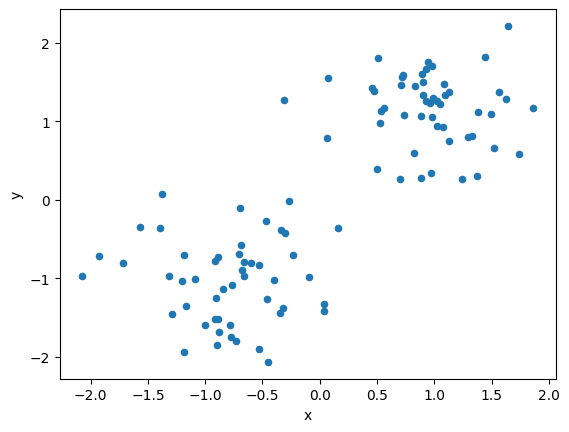
Let us see the data of the clustering problem.

# visualize dataset
df1.plot(kind="scatter", x="x", y="y")
plt.show()

instance_data = {"d": distance_matrix(df1, df1)}

Solving the clustering problem by using OpenJij

We create mathematical model and instance data, so let us solve the clustering problem by using openjij.

pyq_obj, pyq_cache = to_pyqubo(problem, instance_data, {})
qubo, constant = pyq_obj.compile().to_qubo()
sampler = oj.SASampler()
response = sampler.sample_qubo(qubo)
result = pyq_cache.decode(response)

for idx in range(0, N):
    if idx in result.record.solution["x"][0][0][0]:
        plt.scatter(df1.loc[idx]["x"], df1.loc[idx]["y"], color="b")
    else:
        plt.scatter(df1.loc[idx]["x"], df1.loc[idx]["y"], color="r")

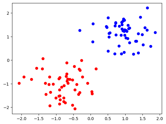
We can see the data is clearly separated by blue and red class.

QBoost

QBoost is a one of the ensemble learning using QA. Ensemble learning involves preparing a number of weak predictors and combining the results of each of these predictors to obtain the final prediction result.

QBoost uses QA to optimize the best combination of learners for a given training data. We handle classification problem in this time.

We define that the set of $D$ training data are $\{\vec x^{(d)}\}(d=1, ..., D)$, corresponding label are $\{y^{(d)}\}(d=1, ..., D), y^{(d)}\in \{-1, 1\}$ and the (function) set of $N$ weak learner is $\{C_i\}(i=1, ..., N)$. For some data $\vec x^{(d)}$, $C_i(\vec x^{(d)})\in \{-1, 1\}$.

Based on the definitions above, the classification labels are as follows.

$${\rm sgn}\left( \sum_{i=1}^{N} w_i C_i({\vec x}^{(d)})\right)$$

Where $w_i\in\{0, 1\} (i=1, ..., N)$, is a weight of each predictor (bool value to adopt or not adopt the predictor for the final prediction).QBoost optimizes the combination of $w_i$ so that prediction matches the training data while erasing the number of weak learners.

Hamiltonian in this problem is as follows.

$$H(\vec w) = \sum_{d=1}^{D} \left( \frac{1}{N}\sum_{i=1}^{N} w_i C_i(\vec x^{(d)})-y^{(d)} \right)^2 + \lambda \sum _i^N w_i$$

The first term represents the difference between weak classifier and the correct label. The second term represents a degree of the number of weak classifier to be employed in the final classifier. $\lambda$ is the regularization parameter that adjust how much the number of weak classifiers affects the total Hamiltonian.

We optimize this Hamiltonian by recognizing the first term as a cost (objective function) and the second term as a constraint.Minimizing with QA allows us to obtain a combination of weak classifiers that best fits the training data.

Preparation of dataset

Let us try QBoost. We use the cancer identification dataset from scikit-learn for training data. For simplicity, we will only use two character types for training: “0” and “1”.

# import libraries
import pandas as pd
from scipy import stats
from sklearn import datasets
from sklearn import metrics

# load data
cancerdata = datasets.load_breast_cancer()
# set the number of training data & test data
num_train = 450

In this time, we consider that feature of noise exists.

data_noisy = np.concatenate(
    (cancerdata.data, np.random.rand(cancerdata.data.shape[0], 30)), axis=1
)
print(data_noisy.shape)

(569, 60)

# convert from label {0, 1} to {-1, 1}
labels = (cancerdata.target - 0.5) * 2

# divide dataset to training and test
X_train = data_noisy[:num_train, :]
X_test = data_noisy[num_train:, :]
y_train = labels[:num_train]
y_test = labels[num_train:]

# from the result of weak learnor
def aggre_mean(Y_list):
    return ((np.mean(Y_list, axis=0) > 0) - 0.5) * 2

Creating Set of Weak Learner

We make weak learner with scikit-learn. In this time, we choose decision stump. Decision stump is a single-layer decision tree. As it will be used as a weak classifier, the features to be used for segmentation are selected randomly (it’s a good understanding that we execute single-layer of random forest).

# import required libraries
from sklearn.tree import DecisionTreeClassifier as DTC

# set the number of weak classifier
num_clf = 32
# set the number of ensembles to be taken out for one sample in bootstrap sampling
sample_train = 40
# set model
models = [DTC(splitter="random", max_depth=1) for i in range(num_clf)]
for model in models:
    # extract randomly
    train_idx = np.random.choice(np.arange(X_train.shape[0]), sample_train)
    # make decision tree with variables
    model.fit(X=X_train[train_idx], y=y_train[train_idx])
y_pred_list_train = []
for model in models:
    # execute prediction with model
    y_pred_list_train.append(model.predict(X_train))
y_pred_list_train = np.asanyarray(y_pred_list_train)
y_pred_train = np.sign(y_pred_list_train)

We look accuracy of all weak learner as the final classifier. Henceforth, we refer to this combination as baseline.

y_pred_list_test = []
for model in models:
    # execute with test data
    y_pred_list_test.append(model.predict(X_test))

y_pred_list_test = np.array(y_pred_list_test)
y_pred_test = np.sign(np.sum(y_pred_list_test, axis=0))
# compute score of prediction accuracy
acc_test_base = metrics.accuracy_score(y_true=y_test, y_pred=y_pred_test)
print(acc_test_base)

0.9411764705882353

Execute QBoost with OpenJij

Let us creater QBoost model.

# set class of QBoost
class QBoost:
    def __init__(self, y_train, ys_pred):
        self.instance_data = {"y": y_train, "C": ys_pred}
        self.qboost_Hamiltonian()
        self.pyq_obj, self.pyq_cache = to_pyqubo(
            self.problem, self.instance_data, {}
        )

    def qboost_Hamiltonian(self):
        problem = jm.Problem("QBoost")
        C = jm.Placeholder("C", dim=2)
        y = jm.Placeholder("y", dim=1)
        N = C.shape[0].set_latex("N")
        D = C.shape[1].set_latex("D")
        w = jm.Binary("w", shape=(N))
        i = jm.Element("i", (0, N))
        d = jm.Element("d", (0, D))
        obj = jm.Sum(
            d,
            (1 / N * jm.Sum(i, w[i] * C[i, d]) - y[d])
            * (1 / N * jm.Sum(i, w[i] * C[i, d]) - y[d]),
        )
        constraint = jm.Constraint("constraint", jm.Sum(i, w[i]))
        problem += obj
        problem += constraint
        self.problem = problem

    def sampling(self, qubo, **kwargs):
        sampler = oj.SASampler(**kwargs)
        response = sampler.sample_qubo(qubo)
        return response

    def decode(self, response):
        return self.pyq_cache.decode(response)

    # set function for converting to QUBO
    def to_qubo(self, norm_param=1):
        # set value of hyperparameter
        self.multiplier = {"constraint": norm_param}
        model = self.pyq_obj.compile()
        return model.to_qubo(feed_dict=self.multiplier)

qboost = QBoost(y_train=y_train, ys_pred=y_pred_list_train)
qboost.problem

$$\begin{alignat*}{4}\text{Problem} & \text{: QBoost} \\\min & \quad \sum_{ d = 0 }^{ D - 1 } \left( \frac{ 1 }{ N } \cdot \sum_{ i = 0 }^{ N - 1 } w_{i} \cdot C_{i,d} - y_{d} \right) \cdot \left( \frac{ 1 }{ N } \cdot \sum_{ i = 0 }^{ N - 1 } w_{i} \cdot C_{i,d} - y_{d} \right) \\\text{s.t.} & \\& \text{constraint} :\\ &\quad \quad \sum_{ i = 0 }^{ N - 1 } w_{i} = 0,\\[8pt]& w_{i_{0}} \in \{0, 1\}\end{alignat*}$$

# make QUBO with lambda=3
qubo = qboost.to_qubo(1)[0]
response = qboost.sampling(qubo, num_reads=100, num_sweeps=10)
result = qboost.decode(response)

Let us check the accuracy in the training/validation data when using a combination of weak classifiers obtained by D-Wave.

accs_train_Dwaves = []
accs_test_Dwaves = []

for solution in result.record.solution["w"]:
    idx_clf_DWave = solution[0][0]
    y_pred_train_DWave = np.sign(
        np.sum(y_pred_list_train[idx_clf_DWave, :], axis=0)
    )
    y_pred_test_DWave = np.sign(
        np.sum(y_pred_list_test[idx_clf_DWave, :], axis=0)
    )
    acc_train_DWave = metrics.accuracy_score(
        y_true=y_train, y_pred=y_pred_train_DWave
    )
    acc_test_DWave = metrics.accuracy_score(
        y_true=y_test, y_pred=y_pred_test_DWave
    )
    accs_train_Dwaves.append(acc_train_DWave)
    accs_test_Dwaves.append(acc_test_DWave)

energies = result.evaluation.energy

We make a graph with energy on the horizontal axis and accuracy on the vertical axis.

plt.figure(figsize=(12, 8))
plt.scatter(energies, accs_train_Dwaves, label="train")
plt.scatter(energies, accs_test_Dwaves, label="test")
plt.xlabel("energy")
plt.ylabel("accuracy")
plt.title("relationship between energy and accuracy")
plt.grid()
plt.legend()
plt.show()

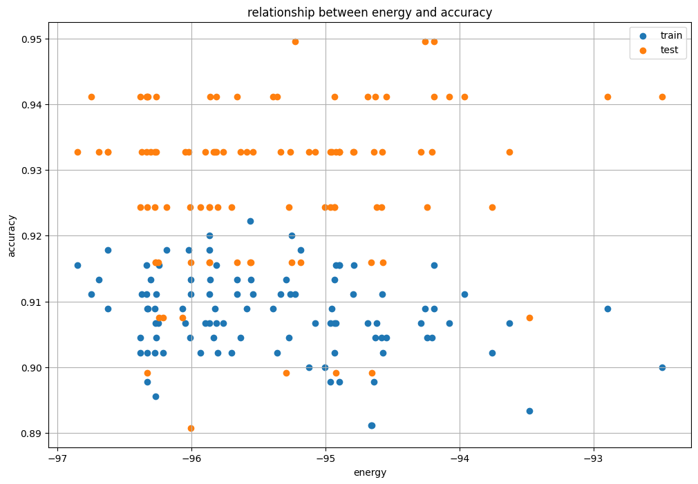
print("base accuracy is {}".format(acc_test_base))
print("max accuracy of QBoost is {}".format(max(accs_test_Dwaves)))
print(
    "average accuracy of QBoost is {}".format(
        np.mean(np.asarray(accs_test_Dwaves))
    )
)

base accuracy is 0.9411764705882353
max accuracy of QBoost is 0.9495798319327731
average accuracy of QBoost is 0.9284033613445378