Clustering with Annealing

This tutorial will cover clustering using PyQUBO and Openjij as an example for an application of annealing.

Clustering

Assuming $n$ is given externally, we divide the given data into $n$ clusters. Let us consider 2 clusters in this case.

Clustering Hamiltonian

Clustering can be done by minimizing the following Hamiltonian:

$$H = - \sum_{i, j} \frac{1}{2}d_{i,j} (1 - \sigma _i \sigma_j)$$

$i, j$ is the sample number, $d_{i,j}$ is the distance between the two samples, and $\sigma_i=\{-1,1\}$ is a spin variable that indicates which of the two clusters it belongs to. Each term of this Hamiltonian sum is:

• 0 when $\sigma_i = \sigma_j$

• $d_{i,j}$ when $\sigma_i \neq \sigma_j$

With the negative on the right-hand side of the Hamiltonian, the entire Hamiltonian comes down to the question to choose the pair of $\{\sigma _1, \sigma _2 \ldots \}$ that maximizes the distance between samples belonging to different classes.

Import Libraries

We use JijModeling for modeling and JijModeling Transpiler for QUBO generation.

import jijmodeling as jm
import numpy as np
import openjij as oj
import pandas as pd
from jijmodeling.transpiler.pyqubo.to_pyqubo import to_pyqubo
from matplotlib import pyplot as plt
from scipy.spatial import distance_matrix

---------------------------------------------------------------------------
ModuleNotFoundError                       Traceback (most recent call last)
Cell In[1], line 1
----> 1 import jijmodeling as jm
      2 import numpy as np
      3 import openjij as oj

ModuleNotFoundError: No module named 'jijmodeling'

Clustering with JijModeling and OpenJij

First, we formulate the above Hamiltonian using JijModeling. Since JijModeling cannot handle the spin variable $\sigma_i$, we rewrite it using the relation $\sigma_i = 2x_i - 1$ so that it can be written in the binary variable $x_i$.

problem = jm.Problem("clustering")
d = jm.Placeholder("d", dim=2)
N = d.shape[0].set_latex("N")
x = jm.Binary("x", shape=(N))
i = jm.Element("i", (0, N))
j = jm.Element("j", (0, N))
problem += (
    -1 / 2 * jm.Sum([i, j], d[i, j] * (1 - (2 * x[i] - 1) * (2 * x[j] - 1)))
)
problem

$$\begin{alignat*}{4}\text{Problem} & \text{: clustering} \\\min & \quad \left( -0.5 \right) \cdot \sum_{ i = 0 }^{ N - 1 } \sum_{ j = 0 }^{ N - 1 } d_{i,j} \cdot \left( 1 - \left( 2 \cdot x_{i} - 1 \right) \cdot \left( 2 \cdot x_{j} - 1 \right) \right) \\& x_{i_{0}} \in \{0, 1\}\end{alignat*}$$

Generating Artificial Data

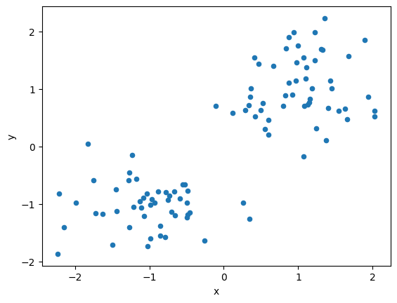
Let us artificially generate data that is linearly separable on a 2D plane.

data = []
label = []
for i in range(100):
    # Generate random numbers in [0, 1]
    p = np.random.uniform(0, 1)
    # Class 1 when a condition is satisfied, -1 when it is not.
    cls =1 if p>0.5 else -1
    # Create random numbers that follow a normal distribution
    data.append(np.random.normal(0, 0.5, 2) + np.array([cls, cls]))
    label.append(cls)
# Format as a DataFrame
df1 = pd.DataFrame(data, columns=["x", "y"], index=range(len(data)))
df1["label"] = label

# Visualize dataset
df1.plot(kind='scatter', x="x", y="y")

<AxesSubplot: xlabel='x', ylabel='y'>

instance_data = {"d": distance_matrix(df1, df1)}

Solving the Clustering Problem using OpenJij

With the mathematical model and data, let us start solving the problem by Openjij. Here we use JijModeling Transpiler.

pyq_obj, pyq_cache = to_pyqubo(problem, instance_data, {})
qubo, constant = pyq_obj.compile().to_qubo()
sampler = oj.SASampler()
response = sampler.sample_qubo(qubo)
result = pyq_cache.decode(response)

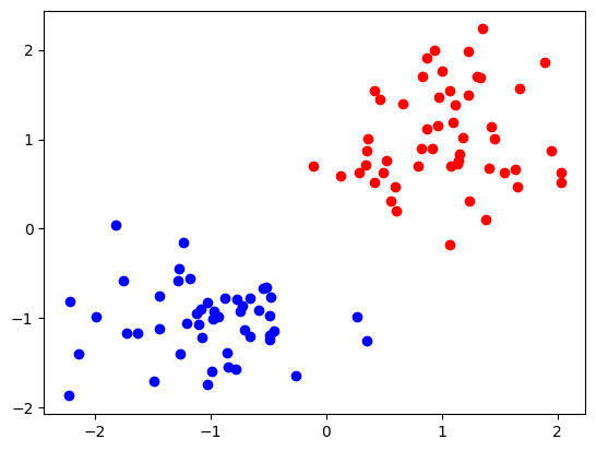
# visualize
for idx in range(0, len(instance_data['d'])):
    if idx in result.record.solution["x"][0][0][0]:
        plt.scatter(df1.loc[idx]["x"], df1.loc[idx]["y"], color="b")
    else:
        plt.scatter(df1.loc[idx]["x"], df1.loc[idx]["y"], color="r")

We see that they are classified into red and blue classes.