HUBO(Higher Order Unconstraint Binary Optimization)

Let us introduce a model with higher-order terms added to the ordinary Ising model. Specifically, we consider the following energy function for the binary variables $\sigma_{i} \in \{-1, +1\}$ or $\sigma_{i} \in \{0, 1\}$:

$$H= c+\sum_{i} h_{i} \sigma_{i}+\sum_{i<j} J_{i j} \sigma_{i} \sigma_{j}+\sum_{i<j<k} K_{i, j, k} \sigma_{i} \sigma_{j} \sigma_{k}+\cdots, \\ i=1,\ldots, N$$

The subscripts $i,j,k,\ldots$ are indices that specify binary variables and take the value of $1\leq i,j,k,\dots \leq N$, and $c$ represents a constant value that corresponds to a zero-order term. The problem of finding variables $(\sigma_{1}, \sigma_{2}, \ldots, \sigma_{N})$ that gives the minimum value of this energy function is called higher-order unconstrained binary optimization (HUBO) or polynomial unconstrained binary optimization (PUBO). In the following, HUBO will be used as the unified term. This type of problem can be regarded as a natural extension of the ordinary Ising model and appears in quantum chemistry. We will show how to solve HUBO using OpenJij in this tutorial.

HUBO can directly be solved by using OpenJij while the method of converting HUBO to QUBO before the computation is also often used. At the end of this tutorial, we will investigate how much the results differ between direct and indirect solution methods for HUBO.

Simple Example of HUBO

For simplicity, we can assume that the problem will only consist of third-order or lower terms with $N=3$ variables. Here we assume that $\sigma_i \in \{-1,+1\}$ is spin variable.

$$H = -\sigma_1 -\sigma_1\sigma_2 +\sigma_1\sigma_2\sigma_3,\;\;\; \sigma_i \in \{-1, +1\}$$

To solve this problem using OpenJij, we first represent the interaction $h_i, J_{ij}, K_{ijk}$ appeared in this energy function to be in python dictionary type. As the following code shows, we set the index specifying spin variables to the key of the dictionary-type, and the interaction to the value.

polynomial = {(1,): -1, (1,2): -1, (1,2,3): 1}

Direct HUBO solving

In general, when solving HUBO, QUBO is solved, which is generated from HUBO by reducing the order of the interaction to the second-order or lower. OpenJij can solve HUBO directly using the simulated annealing without converting HUBO to QUBO by using the following sample_hubo method.

# !pip install openjij

import openjij as oj

# The SASampler method must be selected to use the sample_hubo method.
sampler = oj.SASampler()

# Select sample_hubo method.
# The second argument of the sample_hubo method is the type of variable. 
# "SPIN" or "BINARY" are the options.
# SPIN specifies {-1,1} and BINARY specifies {0,1}.  
response = sampler.sample_hubo(polynomial, "SPIN")
# Check the result.
print(response)

   1  2  3 energy num_oc.
0 +1 +1 -1   -3.0       1
['SPIN', 1 rows, 1 samples, 3 variables]

$\sigma_1=+1,\;\sigma_2=+1,\;\sigma_3=-1$ is obtained as the solution. The energy in this case is -3, which is the optimal solution.

Note that the sample_hubo method can handle non-numeric values as dictionary keys, as shown below.

response = sampler.sample_hubo({('a',): -1, ('a', 'b'): -1, ('a', 'b', 'c'): 1}, "SPIN")
print(response)

   a  b  c energy num_oc.
0 +1 +1 -1   -3.0       1
['SPIN', 1 rows, 1 samples, 3 variables]

For example, ('a', 'b'): -1 means that the interaction between spin a and spin b is -1.

Indirect HUBO solving: solving by QUBO transformation

Another way to solve HUBO is to construct the corresponding QUBO by converting higher-order terms to second or lower-order terms and solving it. This section explains such a method.

To generate QUBO from HUBO, we use D-Wave’s dimod library. Here, the penalty strength set to 5.0 is the penalty for the constraint conditions that arise when converting higher-order interactions to second-order or lower-order interactions. When it is too small, the optimal solution for the generated QUBO will not match the original HUBO, but when it is too large on the other hand, the optimal solution will not be obtained in the first place. In practice, it is difficult to determine how much value to specify. Here we set the value to 5.0 for simplicity.

import dimod

# Generate the corresponding quadratic model by specifying HUBO, the size of penalty strength, and the type of variable.
bqm_dimod = dimod.make_quadratic(poly=polynomial, strength=5.0, vartype="SPIN")
print('zeroth-order term:', bqm_dimod.offset)
print('first-order term:', dict(bqm_dimod.linear))    # bqm.linear converts to python dict
print('quadratic-order term:', dict(bqm_dimod.quadratic)) # bqm.quadratic converts to python dict as well

zeroth-order term: 10.0
first-order term: {1: -3.5, 3: -2.5, '1*3': -2.5, 'aux1,3': -5.0, 2: 0.0}
quadratic-order term: {(3, 1): 2.5, ('1*3', 1): 2.5, ('1*3', 3): 2.5, ('aux1,3', 1): 5.0, ('aux1,3', 3): 5.0, ('aux1,3', '1*3'): 5.0, (2, 1): -1.0, (2, '1*3'): 1.0}

As shown, in addition to the original variables $\sigma_1,\sigma_2,\sigma_3$, two string variables $\sigma_{^"1∗2^"}$ and $\sigma_{^"\rm aux1,2^"}$ appear. In general, converting HUBO to QUBO increases the number of variables and interactions. In this case, the HUBO had 3 variables and 3 interactions, but by converting to the QUBO, the number of variables and interactions increases to 5 and 7, respectively.

We want to solve this QUBO with OpenJij’s simulated annealing, but since OpenJij cannot handle variables that are a mixture of numbers and strings, we need to convert all strings to integers. For this purpose, we use dimod’s method relabel_variables to convert “1∗2” and “aux1,2” to integers.

#Define a function to create a mapping between strings and integers.
def generate_mapping(variables, N):
    mapping = {}
    #Do not change the index of N, which is originally an integer.
    for i in range(1, N+1):
        mapping[i] = i 
    count = N+1
    
    #Convert newly appearing strings to integers.
    for v in variables:
        if type(v) == str:
            mapping[v] = count
            count += 1
    return mapping

# Create a dictionary that represents the correspondence between variables before and after transformation.
mapping = generate_mapping(bqm_dimod.variables, 3)

# Convert the index to an integer starting with 1.
bqm_dimod.relabel_variables(mapping)

print('zeroth-order term:', bqm_dimod.offset)
print('first-order term:', dict(bqm_dimod.linear))    # bqm.linear converts to python dict
print('quadratic-order term:', dict(bqm_dimod.quadratic)) # bqm.quadratic converts to python dict as well
print('Variable correspondence:', mapping) # prints the correspondence between the index after relabeling and the original index.

zeroth-order term: 10.0
first-order term: {1: -3.5, 3: -2.5, 4: -2.5, 5: -5.0, 2: 0.0}
quadratic-order term: {(3, 1): 2.5, (4, 1): 2.5, (4, 3): 2.5, (5, 1): 5.0, (5, 3): 5.0, (5, 4): 5.0, (2, 1): -1.0, (2, 4): 1.0}
Variable correspondence: {1: 1, 2: 2, 3: 3, '1*3': 4, 'aux1,3': 5}

All indices have been converted to integers, and we can solve this QUBO using OpenJij.

# Convert dimod bqm to OpenJij BinaryQuadraticModel.
bqm_oj = oj.BinaryQuadraticModel(dict(bqm_dimod.linear), dict(bqm_dimod.quadratic), bqm_dimod.offset, vartype="SPIN")

# Use the sample method to perform SA.
response = sampler.sample(bqm_oj)
print(response) 

   1  2  3  4  5 energy num_oc.
0 +1 +1 -1 -1 +1   -3.0       1
['SPIN', 1 rows, 1 samples, 5 variables]

The energy obtained here may not correspond to the original energy of HUBO, depending on the value of penalty strength set at 5.0 earlier. Therefore, it is necessary to calculate the energy again. In this case, the original variables were $\sigma_1,\sigma_2,\sigma_3$, so we will calculate the energy using only these spin configurations. Here we note as $\sigma_1=+1,\sigma_2=+1,$ and $\sigma_3=-1$.

# Bake back to the original HUBO solution.
hubo_configuration = {i+1: response.record[0][0][i] for i in range(3)}
print('Corresponding HUBO solution:', hubo_configuration)
print('Energy of the corresponding HUBO solution:', dimod.BinaryPolynomial(polynomial, "SPIN").energy(hubo_configuration))

Corresponding HUBO solution: {1: 1, 2: 1, 3: -1}
Energy of the corresponding HUBO solution: -3.0

Here we have obtained a spin configuration that gives -3 as the energy. This is the optimal solution for this energy function.

This can be verified with dimod’s ExactPolySolver, which is a solver for exact optimal solutions.

# Check the exact optimal solution of the original HUBO.
sampleset = dimod.ExactPolySolver().sample_hising(h = {}, J = polynomial)
print('Optimal solution:',sampleset.first.sample)
print('Corresponding energy:',sampleset.first.energy)

Optimal solution: {1: 1, 2: 1, 3: -1}
Corresponding energy: -3.0

The energy of the optimal solution for the original HUBO is indeed -3.0. Note that the exact solution can be easily obtained in this case because the number of variables was only 3, but it is usually difficult to obtain an exact solution.

Comparing the results of direct and indirect HUBO solving

Finally, let us compare the direct HUBO solution with the indirect HUBO solution where QUBO transformation is used. We run 100 simulations with SA and compare the energies obtained in each simulation.

First, we obtain the energy when using the sample_hubo method.

# Specify the number of simulation times with SA.
num_reads = 100

# SA will be performed independently for num_reads number of times.
# Here, we set it to 100. The default is 1.
response = sampler.sample_hubo(polynomial, "SPIN", num_reads=num_reads)

# Assign the obtained energy to energy_hubo.
energy_hubo = response.energies

Next, we find the energy by using the QUBO transformation. Note that the energy of HUBO must be recalculated each time because there is no guarantee that the magnitude of the previously set penalty strength is appropriate.

response = sampler.sample(bqm_oj, num_reads=num_reads)

# Define a function to recalculate the energy of HUBO from the obtained spin configuration.
def calculate_true_energy(polynomial, response, N):
    energy_quad = []
    for i in range(num_reads):
        hubo_configuration = {j+1: response.record[i][0][j] for j in range(N)}
        energy_quad.append(dimod.BinaryPolynomial(polynomial, "BINARY").energy(hubo_configuration))
    return energy_quad

# Substitute the obtained energy into energy_quad.
energy_quad = calculate_true_energy(polynomial, response, 3)

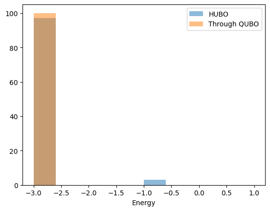
The obtained 100 results are compared in a histogram.

import matplotlib.pyplot as plt
plt.hist(energy_hubo, label='HUBO', range=(-3, 1), bins=10, alpha=0.5)
plt.hist(energy_quad, label='Through QUBO', range=(-3, 1), bins=10, alpha=0.5)
plt.legend()
plt.xlabel('Energy')
plt.ylabel('Frequency')

---------------------------------------------------------------------------
ModuleNotFoundError                       Traceback (most recent call last)
Cell In[12], line 1
----> 1 import matplotlib.pyplot as plt
      2 plt.hist(energy_hubo, label='HUBO', range=(-3, 1), bins=10, alpha=0.5)
      3 plt.hist(energy_quad, label='Through QUBO', range=(-3, 1), bins=10, alpha=0.5)

ModuleNotFoundError: No module named 'matplotlib'

The direct HUBO solution yields slightly more optimal solutions than solving with QUBO transformation. However, in this problem, if penalty strength is set to 1 for example, the solution with QUBO transformation yields more optimal solutions. In other words, the initial value of penalty strength set to 5 is too large as we check below.

# Convert to QUBO with penalty strength set to 1.
bqm_dimod = dimod.make_quadratic(poly=polynomial, strength=1.0, vartype="SPIN")

#Convert the indices to integers and then solve with OpenJij.
bqm_dimod.relabel_variables(mapping)
bqm_oj = oj.BinaryQuadraticModel(dict(bqm_dimod.linear), dict(bqm_dimod.quadratic), bqm_dimod.offset,
vartype="SPIN")
response = sampler.sample(bqm_oj, num_reads=num_reads)

energy_quad = calculate_true_energy(polynomial, response, 3)
# Display the histogram.
plt.hist(energy_hubo, label='HUBO', range=(-3, 1), bins=10, alpha=0.5)
plt.hist(energy_quad, label='Through QUBO', range=(-3, 1), bins=10, alpha=0.5)
plt.legend()
plt.xlabel('Energy')

Text(0.5, 0, 'Energy')

In the current case, the solution by QUBO transformation always provides the optimal solution. Note that the optimal penalty strength value is not known in advance. In this case, the optimal solution is obtained with penalty strength as 1, but determining the appropriate penalty strength for general HUBO is a difficult problem. Another problem is that the QUBO transformation increases the number of variables and interactions. This requires extra memory.

The model we have treated so far as an example is too simple, so let us compare the two solutions with a larger problem. Let us set the number of variables to $N=10$, the interactions to third-order all couplings, and the values to random from -1 to +1.

First, we define the interaction.

import random

N=10
polynomial = {}
for i in range(1, N+1):
    for j in range(i+1, N+1):
        for k in range(j+1, N+1):
            polynomial[(i,j,k)] = random.uniform(-1, +1)

As before, we will perform 100 SAs and compare the energies obtained. The penalty strength for the QUBO transformation is set to 2.

# Solve directly with the HUBO solver.
response = sampler.sample_hubo(polynomial, "SPIN", num_reads=num_reads)
energy_hubo = response.energies

# Solve through the QUBO transform.
bqm_dimod = dimod.make_quadratic(poly=polynomial, strength=2, vartype="SPIN")
mapping = generate_mapping(bqm_dimod.variables, N)
bqm_dimod.relabel_variables(mapping)
bqm_oj = oj.BinaryQuadraticModel(dict(bqm_dimod.linear), dict(bqm_dimod.quadratic), bqm_dimod.offset, vartype="SPIN")
response = sampler.sample(bqm_oj, num_reads=num_reads)
energy_quad = calculate_true_energy(polynomial, response, N)

# Display the histogram.
max_e = max(max(energy_hubo), max(energy_quad))
min_e = min(min(energy_hubo), min(energy_quad))
plt.hist(energy_hubo, label='HUBO', range=(min_e, max_e), alpha=0.5)
plt.hist(energy_quad, label='Through QUBO', range=(min_e, max_e), alpha=0.5)
plt.legend()
plt.xlabel('Energy')
plt.ylabel('Frequency')

Text(0, 0.5, 'Frequency')

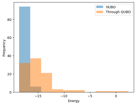
We can see that there is quite a difference in this model: solving HUBO directly yields a lower energy solution. Of course, a more appropriate value of penalty strength could improve the solution by solving with the QUBO transformation, but that is not easy to do.

Summary

The solution method using the QUBO transformation requires preprocessing to convert to QUBO and to determine a parameter called penalty strength. On the other hand, the HUBO solver eliminates the need for such processing, and (at least for the models treated in this study) the solutions obtained are as good as or better than those obtained by the QUBO solver.